Data Pre-Processing
The missing values in the data were visualized using the library missingno. All the columns in the dataset were found to have approximately 2.5% of the data missing. The spread of the data was analyzed and the dataset was found to have columns with varying scales. Thus, making feature scaling an important pre-processing step.
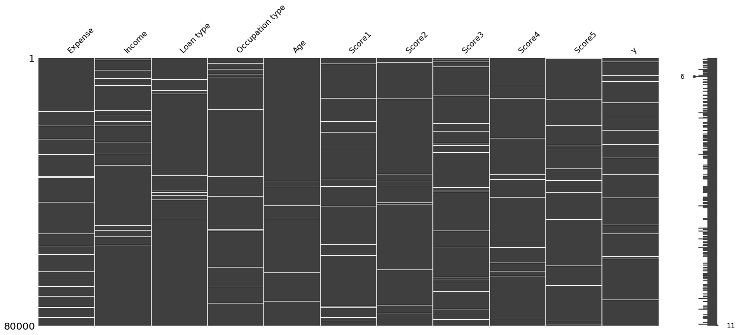
Figure 1
Visualization of missing values in the initial dataset. White horizontal bars indicate missing values.
Data Imputation
Imputation was performed using a Random Forest based method, implemented using the MissForest Imputer. The categorical variables were masked and categorical imputation was performed on them. A total of 6 imputation iterations were performed to completely fill all the missing values in the dataset.
Feature Selection
One-hot encoding of the features - Loan type, Occupation type was done after imputing the dataset and the first category was dropped after the encoding, to ensure that the resulting encoded features are linearly independent.
Correlation
The correlation between the features was calculated and visualized using heatmaps and a cut-off of 0.75 was used to identify all highly correlated features.
The highly correlated features in the dataset were:
| Feature 1 | Feature 2 | Correlation |
|---|---|---|
| Expense | Score5 | 1.000000 |
| Score2 | Score4 | 0.786452 |
| Age | Score2 | 0.780841 |
Multicollinearity
Variance Inflation Factor (VIF) was used to calculate the multicollinearity between the features in the dataset. The VIF of the initial dataset is as follows:
| Features | VIF Factor | Features | VIF Factor |
|---|---|---|---|
| Score5 | 9.051581e+07 | Score3 | 1.894692e+03 |
| Score4 | 5.462307e+07 | Occupation_type_2.0 | 1.282768e+01 |
| Expense | 5.940019e+06 | Occupation_type_1.0 | 7.769822e+00 |
| Score2 | 3.707871e+04 | Loan_type_1.0 | 5.941420e+00 |
| Score1 | 3.267527e+03 | Age | 5.783687e+00 |
| Income | 2.267588e+03 |
From Table 2 it is seen that Score5, Score4 and Expense have a high VIF, a trend similar to what was observed in Table 1.
Data Generation
The dataset was highly imbalanced - with 5247 transactions labeled as defaulted out of 80, 000 transactions. As, several Machine Learning methods are sensitive to imbalanced classes, Synthetic Minority Oversampling Technique (SMOTE)1 was used to generate synthetic data for the defaulted transaction class, so that both classes have the same number of samples.
Prior to the SMOTE data generation, the dataset was split into the train set and the validation set in the ratio 3:1. The samples for class 1, in the train dataset alone were generated using SMOTE. The distribution of samples before and after the SMOTE data generation is as follows:
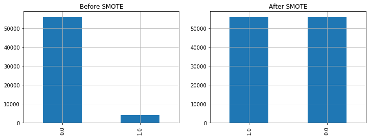
Figure 2
Sample distribution before and after SMOTE data generation. Synthetic data was generated for class 1, so that the number of samples in both classes are the same.
Parameter Tuning
Parameter tuning was carried out using Grid Search with a 5-fold Cross Validation and F1 Score as the scoring function. The parameter tuning was carried out for the following ML models:
- Multi Layered Perceptron (MLP)
- Multi Layered Perceptron (MLP), with Standardized Input Dataset
- Random Forest (RF)
- AdaBoost with Decision Trees as the base classifier.
- Support Vector Machines (SVM)
- Support Vector Machines (SVM), with Standardized Input Dataset
- K-Nearest Neighbors (KNN)
- K-Nearest Neighbors (KNN), with Standardized Input Dataset
- Decision Trees Classifier
- SGD Classifier (linear SVM with Stochastic Gradient Descent)
- Logistic Regression
The performance of the models on the training data, with the best parameter set returned is as shown below:
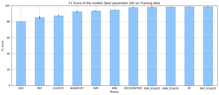
Figure 3
Performance of the models on the training data using the best tuned parameter set returned from GridSearchCV.
Model Selection
All the models above, with the trained parameters and some additional models such as - GaussianNB, BernoulliNB, LDA (Linear Discriminant Analysis) and ExtraTreesClassifier, were implemented on the Validation dataset. The performance of the models is as follows:
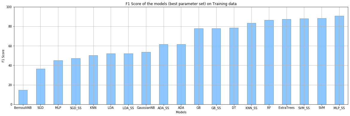
Figure 4
Performance of the models on the training data using the best tuned parameter set returned from GridSearchCV.
From Figure 4, it is noted that the F1-Score of the models - KNN_SS, RF, SVM_SS, ExtraTrees and MLP_SS is greater than 85%.
Final Model - Stacking Classifier
The models that gave an F1-Score greater than 85% were chosen and ensemble classification was done using these chosen models. The ensemble classification methods used are - StackingClassifier with the base model as MLP with Scaled input and VotingClassifier with both hard and soft voting. The results obtained are as follows:
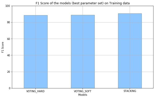
Figure 5
Performance of ensemble models with the models that gave accuracy higher than 85%.
The results obtained are as follows:
| Model | Precision | Recall | F1-Score | Accuracy |
|---|---|---|---|---|
| Stacking Classifier | 91.0 | 90.0 | 91.0 | 99.0 |
| Voting Classfier (Soft) | 89.0 | 89.0 | 89.0 | 99.0 |
| Voting Classfier (Hard) | 89.0 | 88.0 | 88.0 | 98.0 |
The best ensemble model is the Stacking Classifier model, with an F1-Score of 91% and Accuracy of 99%.
References
-
Nitesh V Chawla, Kevin W Bowyer, Lawrence O Hall, and W Philip Kegelmeyer. SMOTE: synthetic minority over-sampling technique. Journal of Artificial Intelligence Research, 16:321–357, 2002. ↩︎
Share:-
-
-
-
-