EfficientNet: Rethinking Model Scaling for Convolutional Neural Networks

Title	EfficientNet: Rethinking Model Scaling for Convolutional Neural Networks
Authors	Mingxing Tan, Quoc V. Le
Institute	Google Research, Brain Team
Link to the Paper	https://arxiv.org/abs/1905.11946
Published on	28 May, 2019

Summary

• This paper proposes a novel compound scaling method that balances between the model’s depth (number of layers), width (number of channels) and resolution (size of the image).
• In addition, they introduce EfficientNet (B0-B7), a family of EfficientNets with SOTA performance in ImageNet top-1, top-5¹. The proposed model stands out for:
  • decrease in the model parameters by $8.4x$
  • decrease in FLOPS by $18x$
  • faster by $6.1x$
    (than when compared to the current SOTA models.)

Introduction

1. Motivation

Model scaling is one of the widely used methods to obtain better accuracies. The most popular scaling methods include:

• depth scaling (i.e.) scaling the number of layers in the model,
• width scaling (i.e.) scaling the number of filters in the model and
• resolution scaling (i.e.) scaling the input size of the model.

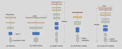
Most models are scaled along one of these dimensions, however, there is no principled way in which all the three dimensions can be simultaneously scaled. Arbitrary scaling of these dimensions would also result in sub-optimal results.

2. Current trends in Scaling

Parameters

Let’s take into consideration the Number of Parameters - Accuracy landscape of the models which have produced SOTA results on the ImageNet dataset.

Year	Model Name	# Parameters	Accuracy (top 1%)
2014	GoogleNet	6.8M	74.8%
2017	SENet	145M	82.7%
2018	GPipe	557M	84.3%

Well, clearly there is an exponential increase in the number of parameters in the models when there is only a marginal increase in the accuracy. So, instead of a blind model scaling, can we implement a systematic scaling method?

Efficiency

ConvNets efficiency came to the forefront when they had to be deployed in smaller devices. Models such as SqueezeNets, MobileNets and ShuffleNets utilize model compression in order to achieve this. However, recent advances in RL and in Neural Architecture Search (NAS) in specific, has opened up possibilities for optimized and efficient model architectures. NAS for larger models also implies a larger design space, higher compute and larger tuning cost. One solution for this would be to build an efficient base model and scale it appropriately.

3. Problems with Existing Approaches

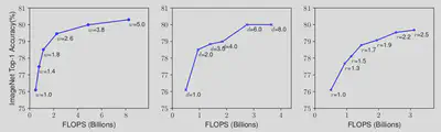
Scaling either one of the dimensions will result in diminishing returns.

The advantage and disadvantage of each scaling technique:

• Depth Scaling:
  • Advantage: Richer and Complex feature extraction.
  • Disadvantage: Vanishing Gradient Problem.
• Width Scaling:
  • Advantage: Extract more fine grained features, easier to train.
  • Disadvantage: Have difficulty capturing higher level features.
• Resolution Scaling:
  • Advantages: Extracts fine grained features.
  • Disadvantage: Larger memory.

From the advantages and disadvantages listed above, we can see that scaling of one dimension is not independent on the other dimensions. If the model resolution is increased, we would need larger receptive fields, and hence, larger depth. Similarly, with higher resolution, in order to extract finer features, we would need larger width. Hence, for optimal model scaling, the depth, width and resolution dimensions should be balanced.

Methods

1. Notation

Through the rest of the paper, the following notation will be used:

• $\mathcal{F_i}$: function that is performed in layer $i$.
• $Y_i = \mathcal{F_i}(X_i)$: $Y_i$ in the output of layer $i$, which has the input $X_i$
• $<H_i, W_i, C_i>$: the dimension of the input $X_i$, where
  • $H_i, W_i$: input spatial dimensions
  • $C_i$: channel dimension

A ConvNet that comprises a base model with $s$ stages is represented as:

$$ \mathcal{N} = ⨀_{i=1}^s \Big(\mathcal{F_i}^{L_i}(X_{<H_i, W_i, C_i>})\Big) $$

where, $⨀$ indicates layer composition and $L_i$ indicates the number of times $F_i$ in repeated in stage $i$

2. Optimization

In our case, we want a model which can provide high accuracies with smaller number of FLOPS. Hence, we would have to perform a combined optimization – optimizing both the accuracy and FLOPS.

Accuracy Optimization

$$ \max_{d, w, r} Accuracy(\mathcal{N}(d, w, r)) $$

$$ s.t. \text{ } \mathcal{N}(d, w, r) = ⨀_{i=1}^s \Big(\mathcal{\hat{F_i}}^{d\cdot \hat{L_i}}(X_{<r\cdot \hat{H_i}, r\cdot \hat{W_i}, w\cdot \hat{C_i}>})\Big) $$

• $d, w, r$ represent Depth, width and resolution.
• $\hat{F_i}, \hat{L_i}, \hat{H_i}, \hat{W_i}, \hat{C_i}$ are parameters set by the base model.
• The base model is decided based on NAS.

FLOPS Optimization

The model FLOPS is optimized using a compound scaling method. $$ \text{depth: } d = \alpha^{\Phi} $$ $$ \text{width: } w = \beta^{\Phi} $$ $$ \text{resolution: } r = \gamma^{\Phi} $$

$$ s.t. \text{ } \alpha\cdot \beta^2\cdot \gamma^2 \approx 2 $$

$$ \alpha\geq 1, \beta^2\geq 1, \gamma^2 \geq 1 $$

$\alpha, \beta$ and $\gamma$ are identified by using a smaller grid search for the base model. Scaling the depth, width and resolution by $\Phi$, would mean that the FLOPS would increase by $2^{\Phi}$.

Combined Optimization

The baseline model $\mathcal{\hat{F}_i}$ is identified using NAS. A multi-objective search, optimizing both the FLOPS and accuracy is performed.

Optimization goal: $ACC(m)\times [FLOPS(m)/T]^w$

where,

• $m$ denotes the model
• $ACC(m)$ denotes the model accuracy
• $FLOPS(m)$ denotes the model FLOPS
• $T$ denotes the target FLOPS
• $w$ denotes the hyperparameter controlling the trade-off between accuracy and FLOPS (value used: $-0.07$)

3. Model

Base Model

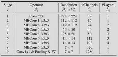
The base model was identified by keeping $\Phi =1$. The values obtained for $\alpha, \beta \text{ and } \gamma$, are $1.2, 1.1, 1.15$. The building block of the model is mobile inverted bottleneck convolution block² and squeeze-and-excitation optimization³ is also used. The obtained parameters are used to build the EfficientNet B0 base model and by varying the value of $\Phi$, EfficientNets B1-B7 are obtained. The baseline model used is as follows:

Training

The specifications of the model training are as follows:

• Optimizer: RMSProp (decay=0.9, momentum=0.9, batch-norm-momentum=0.99)
• Weight decay: 1e-5
• Learning Rate: 0.256 and a decay by 0.97 every 2.4 epochs
• Activation: SiLU (Sigmoid Linear Unit)⁴

Results

1. Proof of Concept

In order to verify that the compound scaling principle works well, it was first used on existing, widely used models such as the MobileNet and ResNet. The results obtained are as follows:

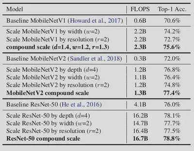
Clearly, compared to a single dimension scaling, the results obtained from compound scaling method proposed were much better.

2. EfficientNets

Now that the compound scaling technique works for existing models, we can apply compound scaling to the Baseline model obtained using NAS and compound scale it. The results obtained using EfficientNets are as follows:

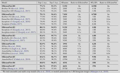
From the results above, we can see that the proposed method + model scaling performs really well – both in terms of parameter efficiency and FLOPS efficiency.

Discussions

Through the course of this paper, we understand the need to have a compound scaling of models as opposed to scaling just a single dimension. The authors went on to show that the proposed compound scaling method, when used on a model, can increase the accuracy by 2.5% than when compared to scaling a single dimension.

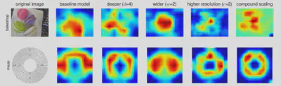
The authors then built an efficient Baseline model B0 using NAS, which can be used for scaling and also showed that their model tends to learn more relevant regions from the input images using Class Activation Maps as shown below:

References