‘Artiphysiology’ reveals V4-like shape tuning in a deep network trained for image classification
| Title | ‘Artiphysiology’ reveals V4-like shape tuning in a deep network trained for image classification |
| Authors | Dean A Pospisil, Anitha Pasupathy, Wyeth Bair |
| Institute | University of Washington |
| Link to the Paper | https://doi.org/10.7554/eLife.38242 |
| Paper Published on | 20 December, 2018 |
Summary
- In this paper, the authors showed that units in CNNs are Translation Invariant (TI) and exhibit Boundary Curvature Selectivity (BCS) too.
- Metrics to quantify both TI and BCS were proposed.
- The variation of the metric values across the layers in a CNN was studied.
- The natural images that maximally drive response in neurons were analyzed.
Introduction
1. Motivation
Deep CNNs perform really well on image recognition and classification. They have a hierarchical structure which is similar to what is found in the visual stream. Different layers in a CNN are shown to have different selectivity.
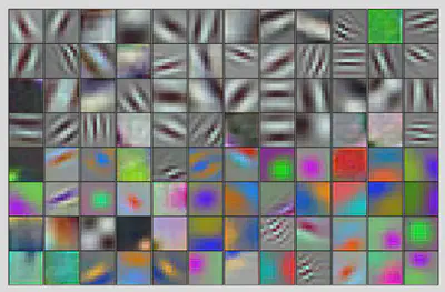
It has been shown that the first layers in CNNs respond to oriented bars and the selectivity of neurons to inputs increases in downstream layers. However, there haven’t been any studies that analyze form-selectivity at an individual neuron level in Artificial Networks.
2. Background
Much of this work is based on an experimental-analysis paper1, where an electrophysiological approach was used to characterize the V4 neurons from rhesus monkeys. In this paper, the authors use a similar approach to characterize units from an artificial network and hence the name - ‘Artiphysiology’.
Methods
1. Model
The artificial neural network (ANN) model AlexNet2 was chosen. The model architecture and receptive field sizes are as follows:
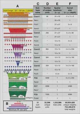
Some important points to note here:
- Input image size: $227\times 227\times 3$
- First layer filter sizes: $11\times 11$
- First layer (conv) RF size: $11\times 11$
- Second layer (conv) RF size: $51\times 51$
- Third layer (conv) RF size: $99\times 99$ and so on
The huge jump in the receptive fields sizes from the first to the second layer is because of the max pooling layer and Conv1 stride length of 4.
2. Dataset
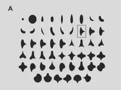
In order to analyze the Boundary Curvature Selectivity, the dataset should consist of variations along these dimensions. The shape dataset proposed in the 2001 paper was used. A total of 51 shapes and 8 rotations (rotational symmetries were discarded), and hence, 362 unique orientations were obtained.
Angular Position and Curvature Modeling (APC Modeling) is used to analyze boundary curvature sensitivity. The main assumption of APC is that the neural response can be explained as a function of product of two Gaussians (one each for angular position and curvature).
3. APC
The mathematical formulation of Angular Position and Curvature Modeling is as follows: $$ R_i = k \max_j \Big[\exp\Big(\frac{-(c_{ij}-\mu_c)^2}{2\sigma_c^2}\Big)\times \exp\Big(\frac{-(a_{ij}-\mu_a)^2}{2\sigma_a^2}\Big)\Big] $$
- $c_{ij}$ is jth curvature for ith shape
- $a_{ij}$ is jth angular position for ith shape
The jth curvature refer to a sample point in a given shape as shown below.
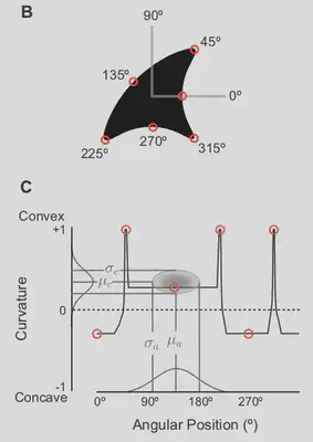
Let us take the example image above. We can see that the shape has:
- concavity from 0 to 45 degrees
- at 45 degrees there is a sharp convexity because of the tip
- the convexity decreases gradually all the way till 225 degrees
- at 225 degrees there is a sharp convexity because of the tip
- this is followed by concavity till 315 degrees
- at 315 degrees, once again there is a sharp convexity because of the tip
- finally there is concavity all the way till 360 degrees
So, once the response is obtained for all the shapes for a given unit, a grid search is performed in order to obtain the values of the 5 parameters. The parameters that resulted in the least difference between the predicted and actual values were chosen.
In addition, the kurtosis value for each unit was calculated. Units outside the kurtosis range for V4 neurons were discarded. Kurtosis is the fourth moment and mathematically it is:
$$K = \frac{1}{n} \sum_{i=1}^n\frac{(x_i-\bar{x})^4}{\sigma^4}$$
Kurtosis can be used to determine how the unit responds. If the value is high, it means that the unit responds for all shapes and has no shape selectivity. If the value is low, it means that the unit doesn’t respond to any shapes or responds to very few shapes.
4. Shape Sizes
The shape sizes had to be set based on layer RF sizes and some additional space is required for translation invariance analysis. Based on RFs, the first layer RF size is too small $(11\times 11)$. When the shapes were reduced to such small sizes, the shape curvatures become distorted. Studying translation invariance would be infeasible with an input image size of $227\times 227$.
So shape size was set to $32\times 32$. This means that if the shape under consideration is a circle, the diameter of the circle was set to 32 pixels. All shape images used are grayscale (all channels: R, G and B have the same value).
5. Translation Invariance
In case of translation invariance, the Classic Receptive Field (CRF) of each unit was identified. CRF is the region where the unit’s response to an input is different from the unit’s response to a blank image.
The center of the shape is varied between 64 and 164 pixels, with a step size of 2. This variation was initially tried in the horizontal direction and later on the vertical direction. The responses to horizontal shifts were highly correlated to the response to vertical shifts.
They also introduced a new metric for Translation Invariance: $$ TI = \frac{\sum_{i\neq j} Cov(p_i, p_j)}{\sum_{i\neq j} SD(p_i) SD(p_j)} $$
Here, $p_i$ is the response at the i\textsuperscript{th} position.
This is very similar to correlation and is better than averaging the correlation over all position response pairs, because in case of averaging, the locations where the response is low will also have equal weightage.
Results
1. Shape Input Response of CNNs
First, we have to verify that the CNN responds to the shape inputs. When the shape inputs were provided to the CNN, the shapes were found to drive the neuron unit responses. On average, CNN units have a similar/greater response than V4 neurons. Distribution of the responses is shown below.
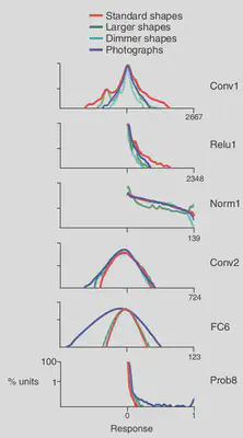
In the initial few layers, the standard shapes drove a wider dynamic range. However, the responses to shapes and photographs became very similar after the normalization layer. Final layer is more responsive to natural images – potentially because the downstream layers learn more categorical information from images so as to classify them.
The response sparsity was analyzed and the points lying outside the kurtosis values of V4 were discarded. Many units were sparse in their response to both shape and natural images.
- 13% units had no response to all shapes.
- 7% units were responsive to only one shape, in only one rotation.
All of these units were also discarded from further analysis.
2. Tuning for Boundary Curvature Selectivity; APC
For each angular position and curvature pair, APC model predictions were obtained. The correlation between the prediction and observed values was calculated. The same was done for V4 neuron recordings. Small statistical correction was done so as to ensure that the number of trails does not affect the inference drawn (V4 Correct). The BCS response obtained are as follows:
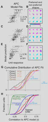
Downstream layer correlations followed the V4 neuron values closely. The leftward shift in V1 could potentially be caused by the whole shape not fitting into the RF. In case of shuffling, the correspondence between predicted and actual recordings is shuffled. The results obtained show that training is important and that the response pattern is very specific to the shapes.
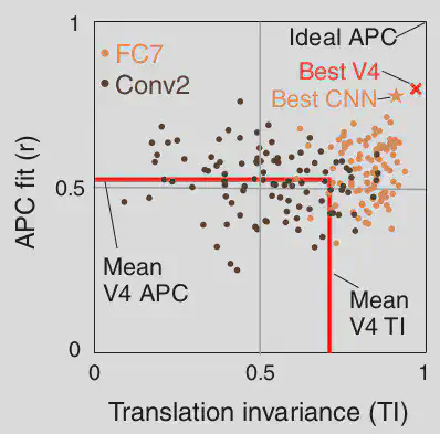
3. Translation Invariance
From experiments, it is known that V4 neurons respond if the input is placed anywhere in the CRF and not just the center of the CRF. Hence, invariance is calculated using the TI metric only in the region where the whole shape is located inside the CRF.
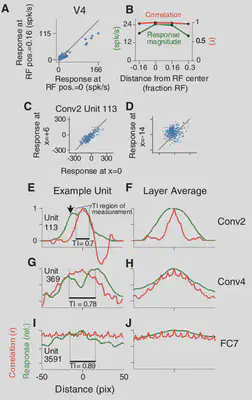
TI increases steadily from lower layers to higher layers, because higher layers have higher RF sizes and become more invariant. Median TI values are higher than that of V4.
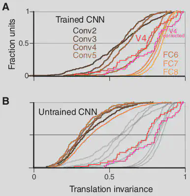
Note that the values in case of untrained networks are to the far left.
4. Visual Preference of Best APC, TI units
After obtaining the TI and APC response of neurons, the natural image patches that maximally drive these neurons were identified. These spahes were provided as inputs to the network and regions that activate these neurons (deconvolutions) were visualized.
Conv 2 Layer
Orientations and conjunctions are expected to be visible in the layer deconvolutions. Texture responses were observed.
-
Max response to 135 degree bars; Min response to 45 degree bars. Mind curvature selectivity is observed.
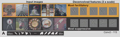
Figure 10: Responses of Conv2Alayer neuron to input image patches; Figure 9 from the paper. -
Example of conjunction. Max response to a conjunction of 135 degree and a vertical bar or vertical bar alone; Min to horizontal lines and 45 degree. Also note the curvature preference.
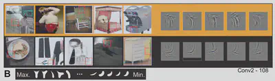
Figure 11: Responses of Conv2Blayer neuron to input image patches; Figure 9 from the paper. -
Example of conjunction. Max response to a conjunction of vertical and horizontal bars; Min to horizontal lines.
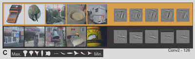
Figure 12: Responses of Conv2Clayer neuron to input image patches; Figure 9 from the paper.
Conv 3 Layer
Encodes object boundaries.
-
Max response to rounded objects like dog paws; Min response to straight edges.
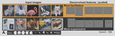
Figure 13: Responses of Conv3Alayer neuron to input image patches; Figure 10 from the paper. -
Example of conjunction of curvature and background. Max response to a conjunction of bright convex objects in dark background; Min response to dark convex object in bright background.
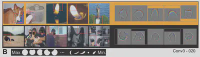
Figure 14: Responses of Conv3Blayer neuron to input image patches; Figure 10 from the paper.
Conv 5 Layer
Encodes object boundaries.
-
Example of conjunction of curvature. Max response to bright convex object; Min response to concave object.
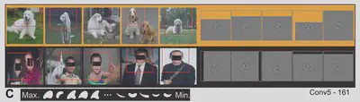
Figure 15: Responses of Conv5Alayer neuron to input image patches; Figure 8 from the paper. -
Example of conjunction of curvature. Max response to pointy objects; Min response to round objects.
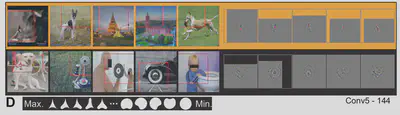
Figure 16: Responses of Conv5Blayer neuron to input image patches; Figure 8 from the paper.
Conclusion
- In this paper, the authors showed that units in CNNs are Translation Invariant (TI) and exhibit Boundary Curvature Selectivity (BCS) too.
- Metrics to quantify both TI and BCS were proposed.
- The variation of the metric values across the layers in a CNN was studied.
- The natural images that maximally drive response in neurons were analyzed.
Remarks
- A much easier way to analyze which responses maximally drive the units would be to perform a gradient ascent from the respective layers3.
- This will be better than choosing image patches and deconvolving them.
References
-
Pasupathy A, Connor CE. 2001. Shape representation in area V4: position-specific tuning for boundary conformation. Journal of Neurophysiology 86:2505–2519. ↩︎
-
Krizhevsky A, Sutskever I, Hinton GE. 2012. ImageNet Classification with Deep Convolutional Neural Networks. In: Pereira F, Burges CJC, Bottou L, Weinberger KQ (Eds). Advances in Neural Information Processing Systems 25. Curran Associates, Inc. p. 1097–1105. ↩︎
-
Erhan, D., Bengio, Y., Courville, A., & Vincent, P. (2009). Visualizing higher-layer features of a deep network. University of Montreal, 1341(3), 1. ↩︎