Shared visual illusions between humans and artificial neural networks

Title	Shared visual illusions between humans and artificial neural networks
Authors	Ari Benjamin, Cheng Qiu, Ling-Qi Zhang, Konrad Kording, Alan Stocker
Institute	University of Pennsylvania
Link to the Paper	https://ccneuro.org/2019/proceedings/0000585.pdf
Published on	September, 2019

Summary

• This paper shows that artificial neural networks (ANNs) trained on natural image datasets also “see” visual illusions.
• In particular, visual illusions pertaining to orientation representation and perception are explored.
• Fisher Information is used to quantify the discriminatory thresholds and perceptual bias.

Introduction

Any resource constrained system should allocate resources efficiently. In case of sensory systems, where the inputs are very noisy, the objective of the system would be to reduce the uncertainty associated with the inputs.

Let’s take for instance the visual system. The visual system should be able to derive essential information from the input. This information could be an object’s color, shape, orientation (absolute and relative if other object’s are also present), texture, curvature and so on. So, if the visual system should have an optimal response to these inputs, the neurons have to be tuned to represent the object and perceive it i.e., derive information from this representation.

One approach of reducing input uncertainty and increasing perceptual accuracy would be allocating resources based on the input distribution.

The system should process frequent variables with higher accuracy than less frequent ones.

Orientation is one such variable, where, there is a higher representation of horizontal and vertical lines in natural images. Hence, we tend to differentiate angles closer to {$0°, 90°$} better. Acute angle changes are the ones that we experience the most. It has been shown that humans tend to overestimate acute angles, while underestimating obtuse angles¹. This estimation bias can be studied and observed through visual illusions such as the Zöllner and Hering Illusions shown below.

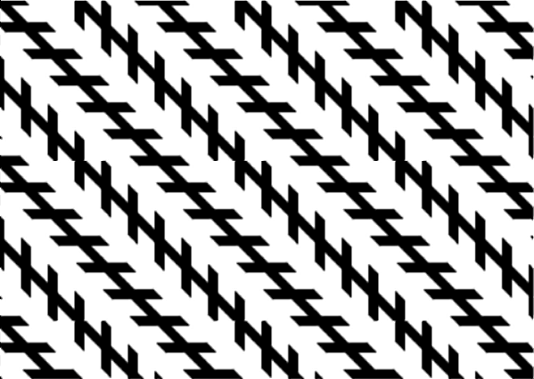
The base lines are actually parallel, but, due to the overestimation of acute angles and underestimation of obtuse angles, we tend to perceive the convergence of the base lines.

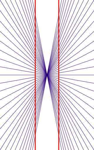
In this case too, due to the estimation bias, we tend to see the base red lines bend when the blue lines are present.

An important question to ask at this point would be – If this disparity arises only because of natural image statistics, can we observe this in artificial networks that are trained on natural images?

It is not obvious that DNNs trained on image classification tasks should share perceptual biases with humans. On the one hand, neural networks may be different from brains, e.g. by having no internal noise. On the other hand, neural networks do have noise related to learning, must represent countless potentially useful variables with a finite number of nodes, and must resolve unavoidable ambiguity.

Methods and Results

Most of the mathematical concepts used in this paper have been previously derived in Wei and Stocker, (2017)². In the following section, the methods used and the corresponding results obtained are simultaneously discussed.

1. Metrics

In order to study the internal representation through the lens of estimation errors, we must study uncertainty estimation. Uncertainty in human perception is quantified using two metrics:

• Discriminatory Threshold (DT)
  • Measure of how well the given stimulus can be distinguished from similar ones.
  • Smaller DT enables us to distinguish between similar inputs better.
  • Hence, for frequently appearing stimuli, the DT has to be very small.
• Perceptual Bias (PB)
  • Measure of how strongly the perceived stimulus deviated from true stimulus value.
  • For frequently appearing stimuli, PB has to be very small.

We can now use these metrics in the context of ANNs to study how they respond.

2. Quantifying Representation

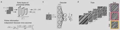
For us to observe representational bias, we must first study how the orientations are understood by the artificial neural networks. Hence, we need the network to “tell” us what angles it “sees”. In order to achieve this, models were trained to estimate the orientation of sinusoidal grating inputs provided to the network.

The network comprised:

• First few layers of the AlexNet (because they are shown to respond to oriented bars)
• A decoder network, which is trained to output two values corresponding to $x, y$

Using the $x, y$ outputs of the model, the orientation angle $\theta$ can be estimated.

3. Quantifying Uncertainty

The paper proposes an approach to quantify uncertainty by using information theory, in particular, Fisher Information. This is because we want to estimate the internal representation associated with this the model, given the neural responses. Hence, in $y = f(\theta)$, we have the values of $y$ (neural responses) and want to see how good an estimate of $\theta$ (internal representation variables) we can get. Fisher Information is mathematically quantified as follows:

$$ J(\theta) = \mathbb{E}[(l’(y|\theta))^2] = -\mathbb{E}[l’’(y|\theta)] = Var[l’(y|\theta)] $$

The detailed proof for the equality can be found here³.

In the equation, $l’(y|\theta)$ is the score function (or) derivative of the log-likelihood function. This means that the fisher information is an estimate of the (absolute) rate of change of the log-likelihood function.

The essence of information theory is that: “An occurrence of a rare event imparts a large amount of information”. Let’s look at this statement in context. Say we have a Gaussian distribution with a very large/small standard deviation (SD) as in the figure below ⁴. What does this tell us about our data?

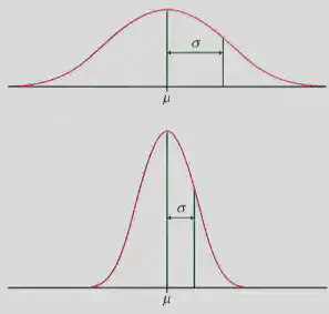
Small variations in the parameter $\mu$ in the small SD case will result in large variations in the likelihood function. This is because, the values are more closely distributed near the mean. As a result, the Fisher Information of the Gaussian (b) will be greater than the Fisher Information of Gaussian (a). Just for the sake of completeness, let us derive this relation for this example. We’ll use the negative expectation of second derivative of likelihood function for this derivation.

$$ f(y, \mu, \sigma) = \frac{1}{\sigma\sqrt{2\pi}} \exp\left( -\frac{1}{2}\left(\frac{x-\mu}{\sigma}\right)^{2}\right) $$

$$ l(y, \mu, \sigma) = \ln(f(y, \mu, \sigma)) = -\frac{\ln 2\pi}{2} - \ln{\sigma} - \frac{(x-\mu)^2}{2\sigma^2} $$

$$ \implies \frac{\partial l}{\partial \mu} = \frac{x-\mu}{\sigma^2} $$

$$ \implies \frac{\partial^2 l}{\partial \mu^2} = -\frac{1}{\sigma^2} $$

Hence, $$ J(\theta) = -\mathbb{E}[l’’(y|\theta)] = \frac{1}{\sigma^2} $$

For smaller $\sigma$, we have larger $J(\theta)$, and vice-versa for larger $\sigma$.

Now, let’s use this to quantify the Discriminatory Threshold (DT) and Perceptual Bias (PB). As mentioned in the Introduction, we would want both DT and PB to be small for frequent stimuli. In Wei and Stocker, (2017)², it has been proved that

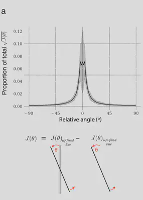
• The distribution of orientations in the input image, $p(\theta)$, is proportional to $\sqrt{J(\theta)}$, (i.e.) $p(\theta) \propto \sqrt{J(\theta)}$
• The Discriminatory Threshold (DT, $D(\theta)$) is inversely proportional to $p(\theta)$, (i.e.) $D(\theta) \propto (J(\theta))^{-0.5}$.
• The Perceptual Bias (PB, $b(\theta)$) is inversely proportional to $p(\theta)^2$, (i.e.) $b(\theta) \propto (J(\theta))^{-1}$.
• Under the assumption that the noise is independent Gaussian noise, $J(\theta)$ can be calculated as: $J(\theta) = ||\frac{\partial f}{\partial \theta}||^2_2$.

The variation of these parameters across different orientations were observed and the results obtained are as follows:

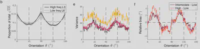
The model was trained in three regimes:

• First: Estimate the absolute orientation of input gratings.
• Second: Estimate the relative orientation of an input. In the presence of two lines, one fixed and the other rotating, the relative angle is estimated.
• Third: Estimate orientation at the pixel level. Given an input, the network has to estimate the orientation at each pixel. In this case, the base model used was changed to VVGNet.

When the $J(\theta)$ of the relative orientation is calculated, the $J(\theta)$ obtained is subtracted from the $J(\theta)$ of rotating line without the fixed line. This ensures that the Fisher Information values mirror those of the relative angle and not the absolute angle.

4. Orientation Bias

After estimating the response of the network to absolute and relative angles, the network is now tested on visual illusions. For the network to be able to tell us what it sees, it should be able to estimate the orientation at each pixel (final training regime). Here, the decoder is modified accordingly.

The model is provided inputs of the visual illusions and the decoder response is color coded based on the perceived orientation. The results are as follows:

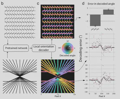
In the figure above, error is calculated as: $(true - predicted)$.

Case 1: Zöllner Illusion

Observing the error in case of the left and right hatched lines, we can see that:

• In right hatching, the network tends to overestimate the acute angles, resulting in a negative error as the $predicted$ orientation is greater than the $true$ orientation.
• In case of left hatching, the network tends to underestimate the obtuse angles, resulting in a positive error as the $predicted$ orientation is lesser than the $true$ orientation.

Hence, the network “sees” the Zöllner illusion!

Case 2: Hering Illusion

Observing the error in case of the top and bottom horizontal lines, we can see that:

• In the top line, the network tends to underestimate the obtuse angles initially, estimate the vertical line precisely and overestimate the acute angles. This variation is seen clearly in the error patterns, which increases initially, is exactly zero at 90° and becomes negative after that.
• In the bottom line, the network tends to overestimate the acute angles initially, estimate the vertical line precisely and underestimate the obtuse angles. This variation is seen clearly in the error patterns, which decreases initially, is exactly zero at 90° and becomes positive after that.

Hence, the network also “sees” the Hering illusion!

Conclusion

Through the paper, we saw that an artificial network trained on natural images, learns representations which reflect the statistics of natural images. We studied this representation using metrics such as the Fisher Information, Discriminatory Threshold and Perceptual Bias. At the end, we learnt that given the natural image statistics, an Artificial Network can also see visual illusions.

Remarks

• As the main aim of the paper was to study orientation sensitivity, the first few layers were only taken into consideration. However, it would be interesting to observe how the metrics vary when additional layers are taken into consideration.
• As higher layers respond to complex patters, will we be able to observe preferences for orientation conjunctions and specific shapes in the higher layers?
• Can we then generalize this principle of efficient coding to explain other classes of illusion, say for instance, color constancy?
• Given that this paper was a conference submission, the methods were not described in detail. Upon a detailed paper being published, this summary will be revised.

References